The carbon budget has become synonymous with climate policy rhetoric. The general story is that we have a limited time before the carbon budget is used leading to climate disaster, we must act quickly, and fossil fuels must stay in the ground.

All quite true, but many are fast learning that the carbon budget is rather malleable. There is no magic number, but rather a dauntingly large range. The carbon budget is not a unique property of the climate system, but rather, something that is shaped by socioeconomic assumptions, climate uncertainties, and user choices.

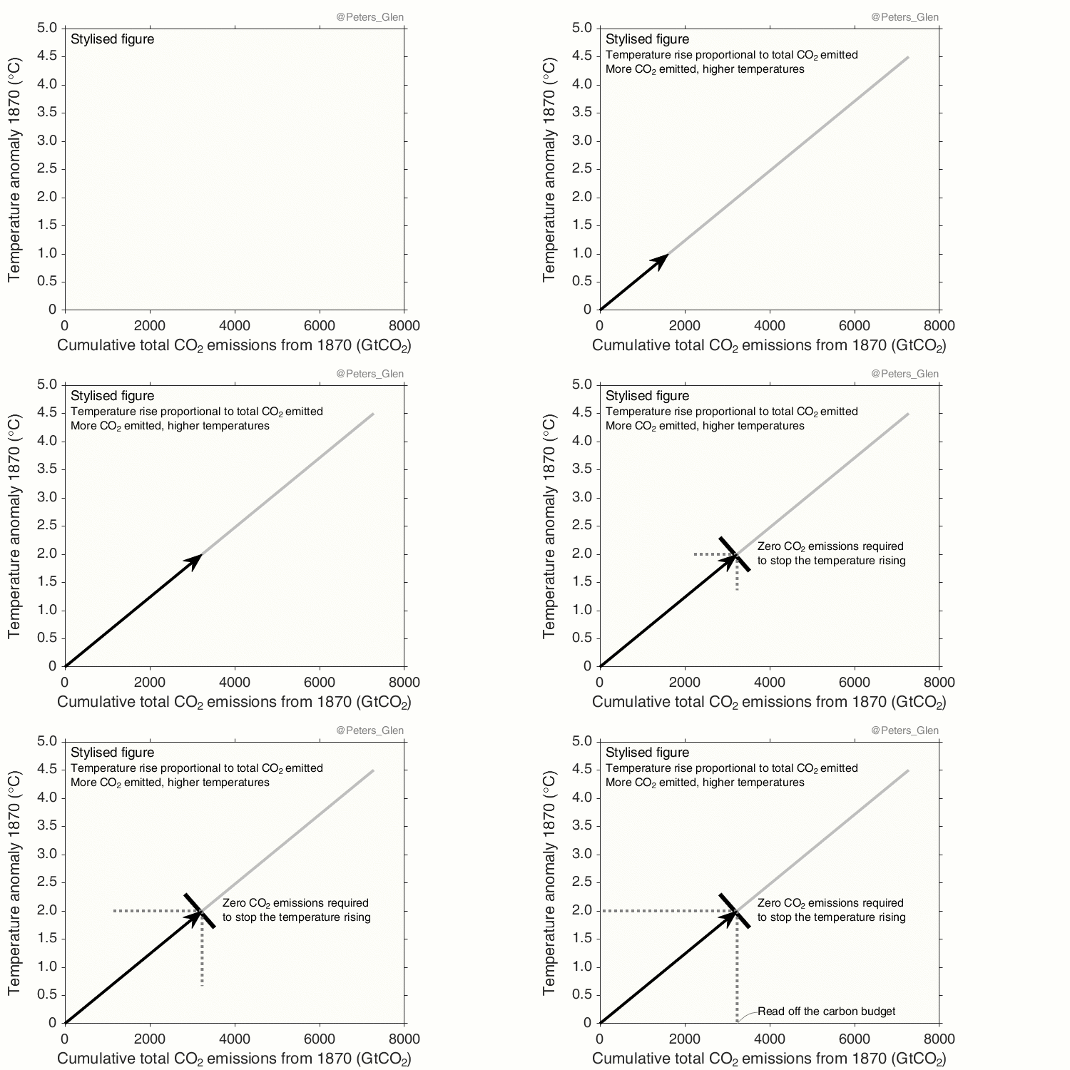
The carbon budget originates out of the near-linear relationship between the temperature anomaly and cumulative carbon dioxide emissions. It is a very powerful concept, hopefully expressed in the following stylised animation:

• Climate change is a cumulative problem: the total carbon dioxide emitted over time matters, not the emissions in any given year;
• The relationship is near-linear, which is remarkable given the non-linearities in the climate system (two opposing non-linearities cancel, leading to near-linear).
• The temperature will keep rising until carbon dioxide is no longer emitted;
• Emitting more today, means emitting less later, and vice-versa;
• We must get to zero carbon dioxide emission;
• If we put too much carbon dioxide into the atmosphere, we have to take it back out (net-negative emissions).

Life is never so simple…

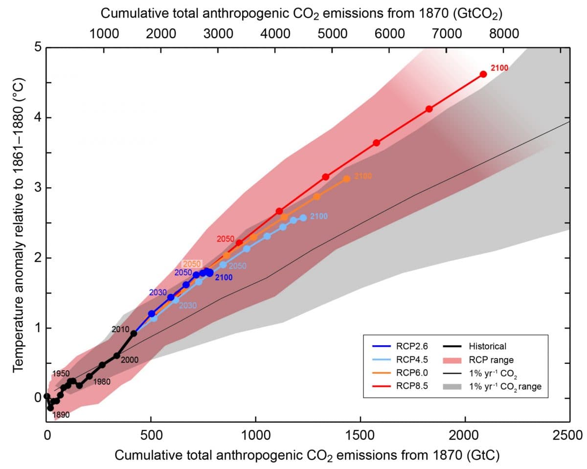
The original figure presented by the IPCC (AR5 WG1 Figure SPM.10) clearly shows that there is significant uncertainty, the relationship is only near linear, and non-CO₂ emissions effect the relationship (orange versus grey shaded regions). There are also alternative definitions of the carbon budget, and as you get closer to the desired temperature level, the uncertainty grows.

A risky metric

While the carbon budget has some nice features to communicate the climate challenge, excellent for an elevator pitch, the practical policy utility of the concept is less obvious due to the persistent uncertainties.

Climate scientists happily fess up and defend the (irreducible) uncertainty in the climate sensitivity, but this has not yet happened with the carbon budget. Rarely is a carbon budget range presented, even though its range is closely connected to that of the range of the climate sensitivity.

The constantly changing carbon budget is, in my view, a simple outcome of the physical, social, and user uncertainties inherent with the carbon budget concept. Since the carbon budget for 1.5°C is diminishingly small, these uncertainties are amplified. The uncertainties still exist for a 5°C carbon budget, but they are relatively small compared to the size of the carbon budget.

Carbon budgets are easy, in principle

Climate scientists noticed that the temperature response was largely independent of the emission pathway. What mattered most was the total amount of carbon emitted, not the pathway. In mathematics terms, the area under the curve mattered, not the shape of the curve.

We can use stylized figures to show this. Here I take the median of «below 1.5°C» scenarios available in the literature and do some high school mathematics. I integrate the curves. Net-negative emissions (below the zero line) make defining the carbon budget ambiguous, and this is shown by the different colours and discussed below.

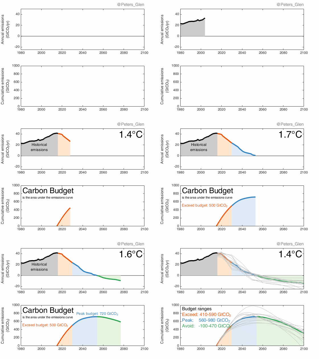
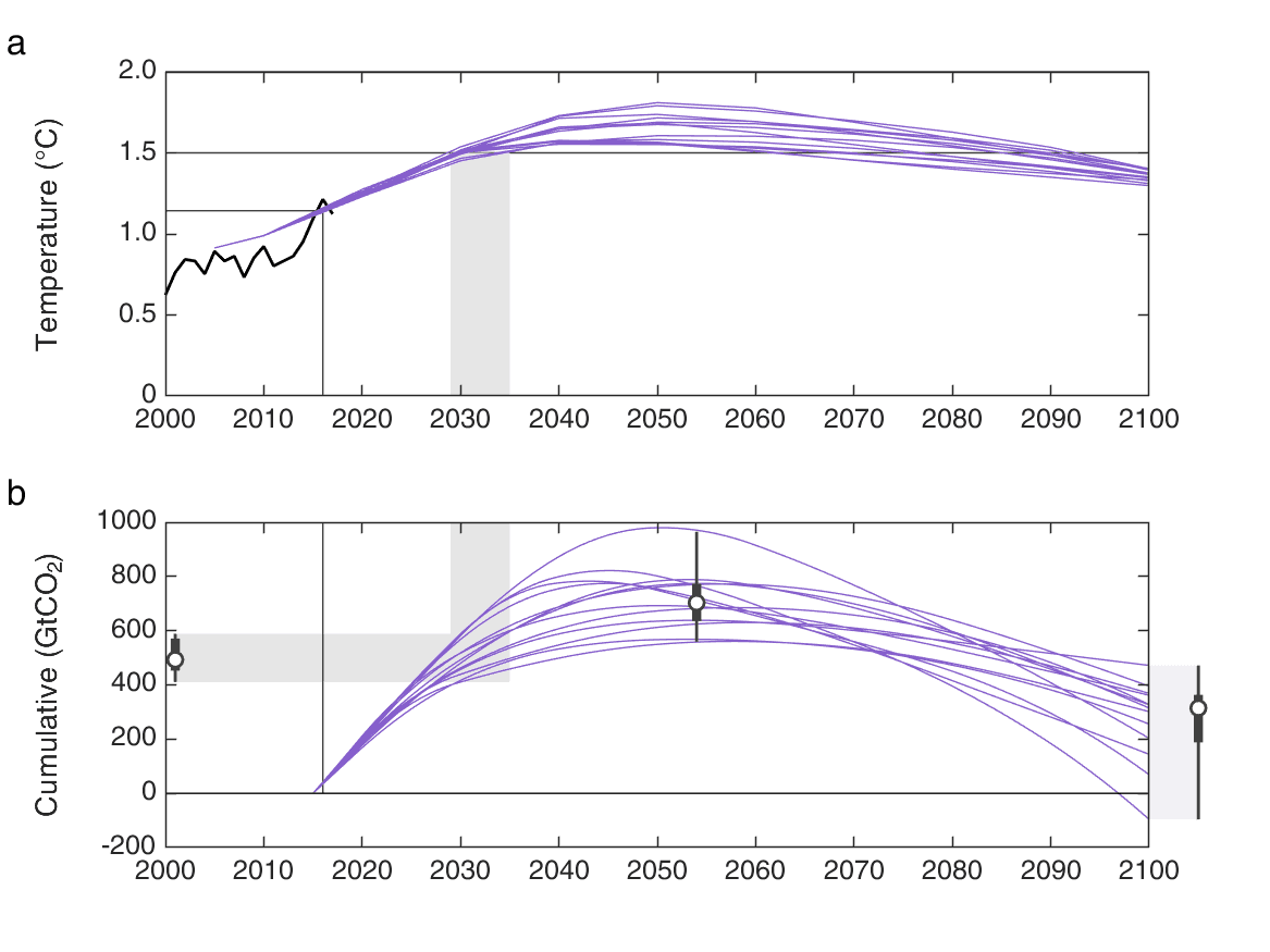
Let’s go a step deeper, to understand how these carbon budgets were defined. The following figures shows the temperature anomaly (top) and the cumulative emissions (bottom). Here are the carbon budget definitions:

• Exceedance: In the top panel, 1.5°C is exceeded by all the scenarios, in the 2030s, and the carbon budget is the emissions from today until the year 1.5°C is exceeded. The percentiles are shown to the left of the figure (follow the grey shading): median: 500GtCO₂, 25-75% range is 450-570GtCO₂, and the full range is 410-590GtCO₂.
• Peak (at the year of zero emissions): This is the maximum value of the cumulative emissions, rather easy to define, but a different year for each scenario. The range is shown at the median zero year across all scenarios (2054), with percentiles: median: 720GtCO₂, 25-75% range is 640-770GtCO₂, and the full range is 560-980GtCO₂.
• Avoidance: This is the cumulative emission up to a given year, taken here as 2100 (somewhat arbitrarily because this is where the scenarios end). The range is shown after 2100, with percentiles: median: 310GtCO₂, 25-75% range is 190-360GtCO₂, and the full range is -100-470GtCO₂.

The details…

The first point to highlight is that each scenario leads to a different carbon budget. All these scenarios have been run through the same simple climate model, MAGICC, so they have the same background climate system. It is the emission pathway, and particularly the non-CO₂ pathways, that lead to the different carbon budgets (for a given definition).

The exceedance carbon budget is easy to define and have the narrowest range across scenarios, probably due to the large inertia in the climate system. Due to the cumulative emissions relationship, one could argue that the exceedance carbon budget is similar in size to the carbon budget when the temperature goes back below 1.5°C in the 2070s or 2080s. This will not be strictly true, because of non-CO₂ emissions, but worth noting! The exceedance budget is often used in Earth System Model estimates of carbon budgets.

The peak carbon budget is easy to define and corresponds approximately to the year of peak temperatures. However, even though these are all «below 1.5°C» scenarios, since they first exceed 1.5°C before returning (peak and decline), the maximum temperature is between 1.6–1.8°C, well over 1.5°C. If we used the peak carbon budget, 1.5°C would be permanently exceeded. In a sense, the peak carbon budget only tells half the story. It does not reveal the need for negative emissions. With a peak budget we also begin to see more variation across the carbon budgets in different models and scenarios.

The avoidance carbon budget is a little arbitrary to define, and I have integrated all the way to 2100 when the scenario ends, as done in Rogelj et al. The avoidance carbon budgets are much smaller as they bring in the negative emissions required to stay «below 1.5°C» (green in the above figures). The avoidance carbon budget gets smaller over time as long as emissions remain net negative. If you wait long enough, we can technically cool the planet below pre-industrial levels…

The role of non-CO₂ emissions

The following bar chart shows the cumulative emissions for each of the 1.5°C scenarios, decomposed into the different definitions, corresponding to the colours in the animation above. The orange is the exceedance carbon budget, the orange plus blue is the peak carbon budget, and the orange, blue, plus green is the avoidance carbon budget (black dot).

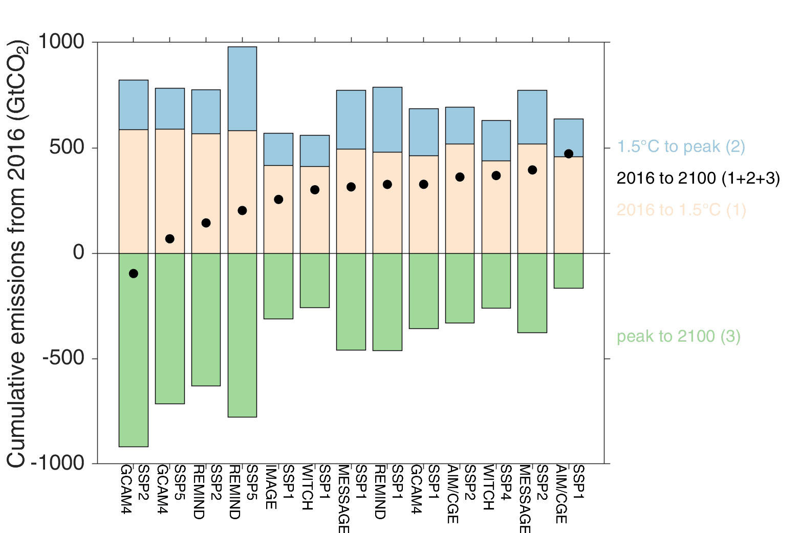
The variation in the carbon budgets, avoidance carbon budgets in particular, are driven by non-CO₂ emissions, which in turn is driven by the cumulative net-negative emissions (green). This can be seen in more detail by comparing Figures 1c and 1f in Rogelj et al, but also indicated in van Vuuren et al. It is also possible to show the relationship by performing regressions on non-CO₂ forcing and cumulative emissions.

The key point is that the net-negative emissions (green) correlates strongly with non-CO₂ radiative forcing: Less non-CO₂ emissions, less demand for negative emissions.

Take home messages

All the carbon budget definitions reveal a part of the puzzle, but no carbon budget reveals all the pieces of the puzzle. To complete the puzzle we need the full emission pathway, not the carbon budget! The carbon budget is simply too aggregated an indicator to be useful for policy.

It is important to note that there are different definitions, with rather significant differences in carbon budgets. This means, explicitly or implicitly, people may make choices which lead to bigger or smaller carbon budgets. There is no scientifically unique way to define a carbon budget, unfortunately.

It is important to note that carbon budgets depend strongly on non-CO₂ emission pathways, even though they are carbon budgets. The relationship between carbon dioxide and non-CO₂ has always been an important discussion in climate policy, but that has not been recognized sufficiently in the carbon budget literature (though this is now changing).

In the commentary, Beyond Carbon Budgets, I bring up four main issues important for carbon budgets:

• How temperature is defined;
• Definitions (discussed above);
• Non-CO₂ (partially discussed above);
• The way uncertainties are expressed.

Read the commentary for more details, and don’t miss the one by Oliver Geden on the political dimensions.